Graph Markov Network

This is a post introducing a Graph Markov Network structure for dealing with spatial-temporal data forecasting with missing values.

Problem Definition
Graph Markov Process
- Handling Missing Values in Graph Markov Process
Graph Markov Network
Code
Reference

Traffic forecasting is a classical task for traffic management and it plays an important role in intelligent transportation systems. However, since traffic data are mostly collected by traffic sensors or probe vehicles, sensor failures and the lack of probe vehicles will inevitably result in missing values in the collected raw data for some specific links in the traffic network.

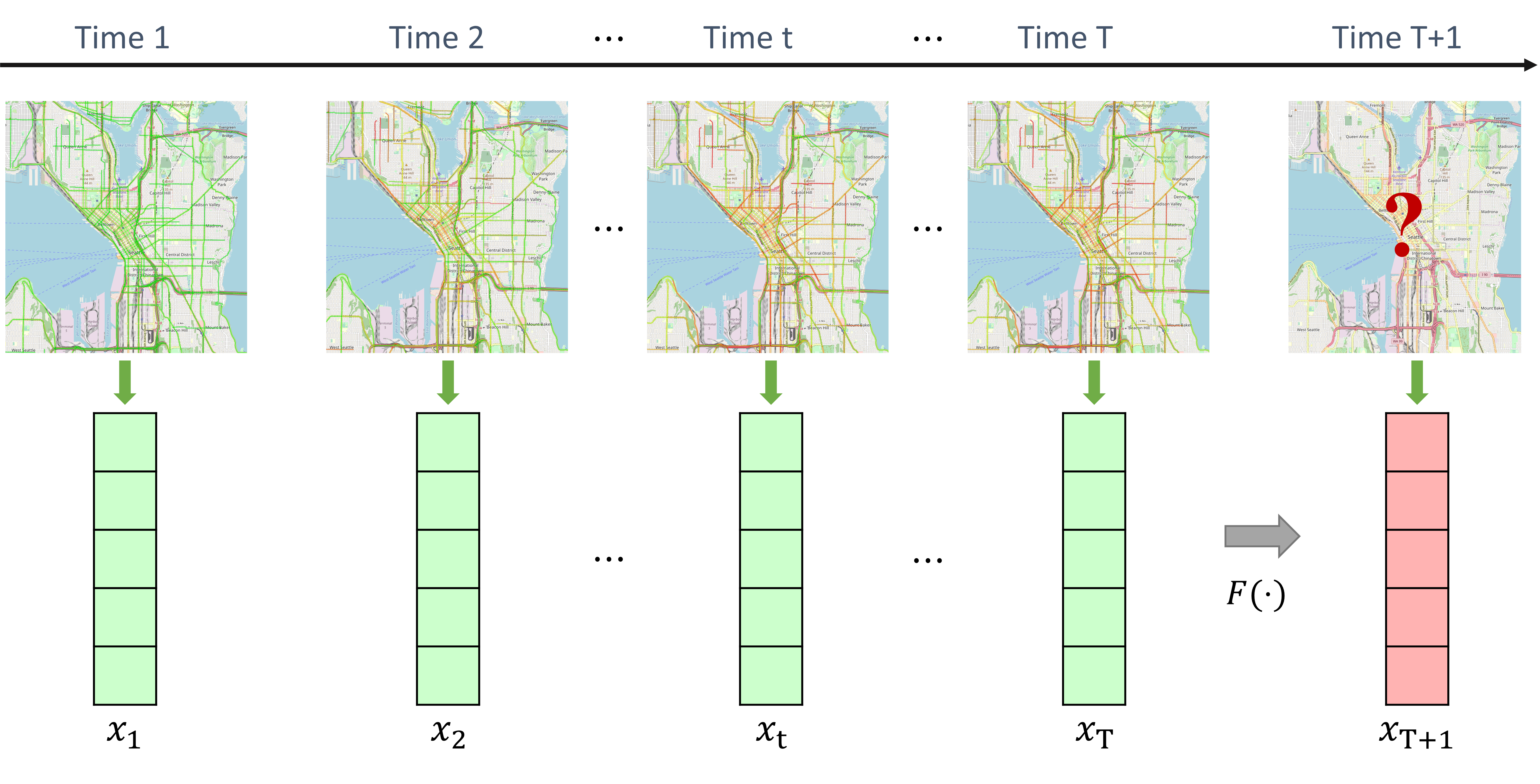
A traffic network normally consists of multiple roadway links. The traffic forecasting task targets to predict future traffic states of all (road) links or sensor stations in the traffic network based on historical traffic state data. The collected spatial-temporal traffic state data of a traffic network with $S$ links/sensor-stations can be characterized as a $T$ -step sequence $[x_1,x_2,...,x_t,...,x_T] \in \mathbb{R}^{T \times S}$ , in which $x_t \in \mathbb{R}^{S}$ demonstrates the traffic states of all $S$ links at the $t$ -th step. The traffic state of the $s$ -th link at time $t$ is represented by $x_t^s$ .

Here, the superscript of a traffic state represents the spatial dimension and the subscript denotes the temporal dimension.

Problem Definition

Traffic Forecasting

The short-term traffic forecasting problem can be formulated as, based on $T$ -step historical traffic state data, learning a function $F(\cdot)$ to generate the traffic state at next time step (single-step forecasting) as follows:

$F([x_1,x_2...,x_T]) = [x_{T+1}]$

Problem definition 1

Learning Traffic Network as a Graph

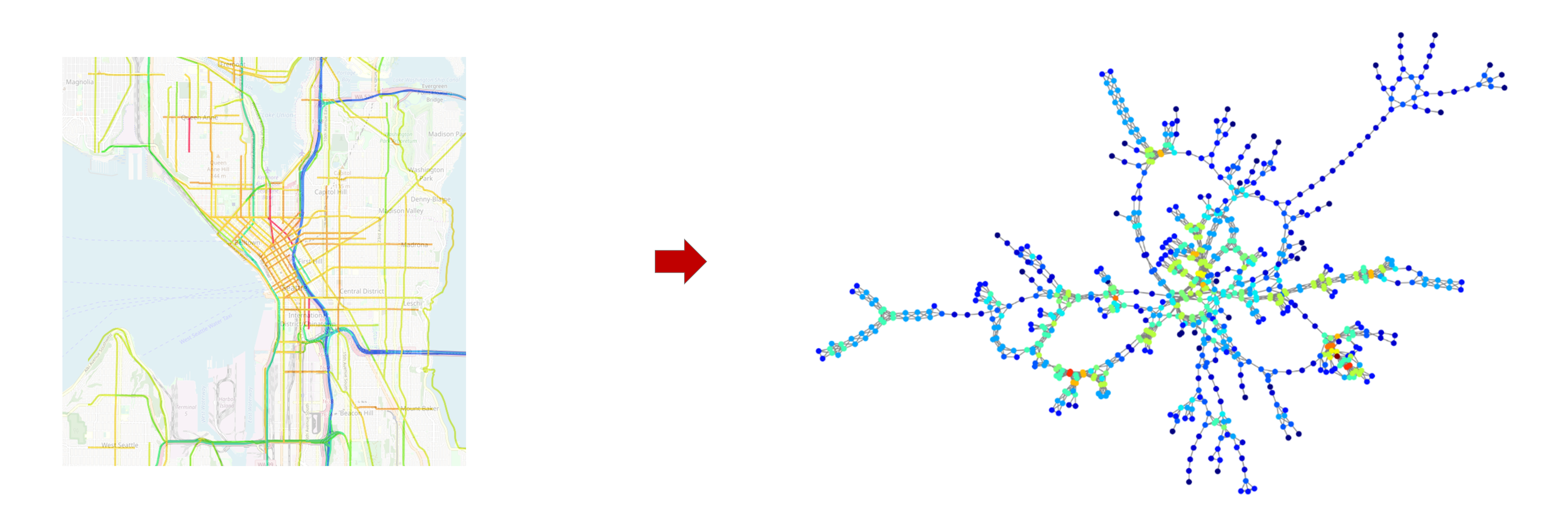
Since the traffic network is composed of road links and intersections, it is intuitive to consider the traffic network as an undirected graph consisting of vertices and edges. The graph can be denoted as $\mathcal{G}=(\mathcal{V}, \mathcal{E}, \mathcal{A})$ :

$\mathcal{V}$ : a set of vertices $\mathcal{V}=\{v_1,...,v_S\}$ .
$\mathcal{E}$ : a set of edges $\mathcal{E}$ connecting vertices.
: an adjacency matrix, a symmetric (typically sparse) adjacency matrix with binary elements, in which denotes the connectedness between nodes and .
- To characterize the vertices’ self-connectedness, a self-connection adjacency matrix is denoted as $\mathbf{A} = \mathcal{A} + I$ , i.e. $\mathbf{A}_ {i,i}=1$ , implying each vertex in the graph is self-connected. Here, $I \in \mathbb{R}^{S \times S}$ is an identity matrix.
- Based on $\mathcal{A}$ , a graph degree matrix ( $\mathcal{D} \in \mathbb{R}^{S \times S}$ ) describing the number of edges attached to each vertex can be obtained by $\mathcal{D}_ {i,i} = \sum_{j=1}^S \mathcal{A}_ {i,j}$ .
- The connectedness of the graph vertices can also be encoded by the Laplacian matrix ( $\mathcal{L}$ ), which is essential for spectral graph analysis. The combinatorial Laplacian matrix is defined as $\mathcal{L} = \mathcal{D}-\mathcal{A}$ , and the normalized definition is $\mathcal{L} = I - \mathcal{D}^{-1/2}\mathcal{A}\mathcal{D}^{-1/2}$ . Since $\mathcal{L}$ is a symmetric positive semi-definite matrix, it can be diagonalized as $\mathcal{L}=U\Lambda U^T$ by its eigenvector matrix $U$ , where $U=[u_0, u_1,..., u_{S-1}] \in \mathbb{R}^{S \times S}$ and $\Lambda = \operatorname{diag}(\lambda_0, \lambda_1,..., \lambda_{S-1})\in \mathbb{R}^{S \times S}$ is the corresponding diagonal eigenvalue matrix satisfying $\mathcal{L}u_i = \lambda_i u_i$ .

Problem definition 2

Given the graph representation of the traffic network, the traffic forecasting problem can be reformulated as

$F({\color{#C00000}{\mathcal{G}}},[x_1,x_2...,x_T]) = [x_{T+1}]$

Traffic Forecasting with Missing Values

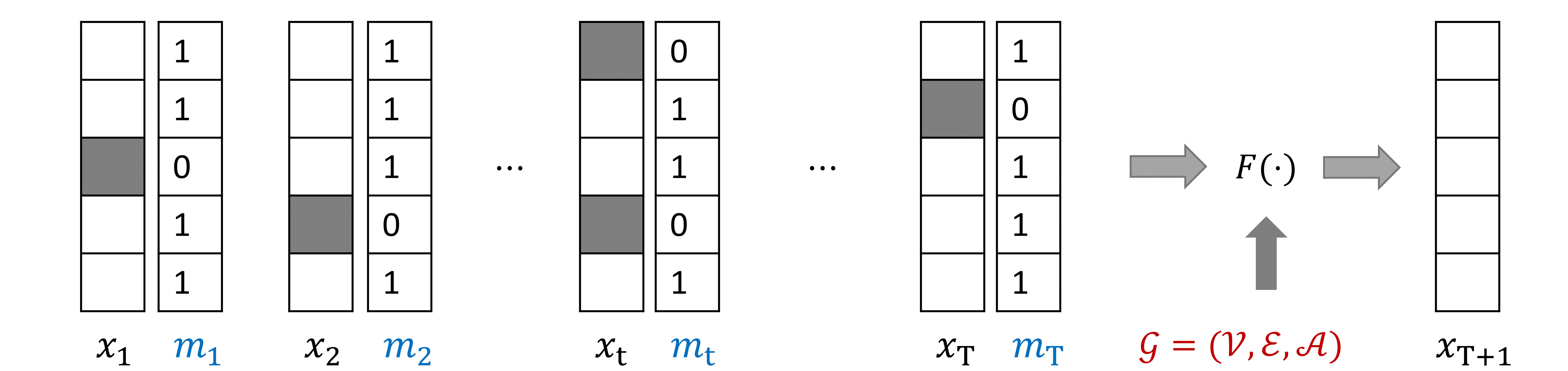
Traffic state data can be collected by multi-types of traffic sensors or probe vehicles. When traffic sensors fail or no probe vehicles go through road links, the collected traffic state data may have missing values. We use a sequence of masking vectors $[m_1,m_2,...,m_T] \in \mathbb{R}^{T \times S}$ , where $m_t \in \mathbb{R}^{S}$ , to indicate the position of the missing values in traffic state sequence $[x_1,x_2,...,x_T]$ . If $x_t^s$ is observed $m_t^s = 1$ , otherwise $m_t^s = 0$ .

Taking the missing values into consideration, we can formulate the traffic forecasting problem as follows

$F({\color{#C00000}{\mathcal{G}}},[x_1,x_2...,x_T],{\color{#0070C0}{[m_1,m_2...,m_T]}}) = [x_{T+1}]$

Problem definition 3

Graph Markov Process

A traffic network is a dynamic system and the states on all links keep varying resulted by the movements of vehicles in the system. We assume teh transitions of traffic states have two properties

Markov Property: The future state of the traffic network $x_{t+1}$ depends only upon the present state $x_t$ , not on the sequence of states that preceded it. Taking $X_1, X_2, ... ,X_{t+1}$ as random variables with the Markov property and $x_1,x_2,...,x_{t+1}$ as the observed traffic states. The Markov process can be formulated in a conditional probability form as

$Pr(X_{t+1} = x_{t+1} | X_1 = x_1, X_2 = x_2, ..., X_t = x_t)=Pr(X_{t+1} = x_{t+1} | X_t = x_t)$

where $Pr(\cdot)$ demonstrates the probability. It can be formulated in the vector form as

$x_{t+1} = {\color{#0070C0}{P_t}} x_t$

where $P_t \in \mathbb{R}^{S\times S}$ is the transition matrix and ${(P_t)}_ {i,j}$ measures how much influence $x_t^j$ has on forming the state $x_{t+1}^i$ .

The time interval $\Delta t$ between two consecutive time steps of traffic states will affect the transition process. Thus, a decay parameter $\gamma \in (0,1)$ is multiplied to represent the temporal impact on transition process as

$x_{t+1} = \gamma {\color{#0070C0}{P_t}} x_t$

Graph Localization Property: We assume traffic state of a link 𝑠 is mostly influenced by itself and neighboring links. This property can be formulated in a conditional probability form as

$Pr(X_{t+1} = x_{t+1}^u | X_t = x_t) = Pr(X_{t+1} = x_{t+1}^u | X_t = x_t^v, v \in \mathcal{N}(u))$

where the superscripts $u$ and $v$ are the indices of graph links (road links). The $\mathcal{N}(u)$ denotes a set of one-hop neighboring links of link $u$ and link $u$ itself. Its vector form can easily represented by

$x_{t+1} = {\color{#C00000}{A}} x_t$

Graph Markov Process: By incorporating the Markov property and the graph localization property, the traffic state transition process is defined as a graph Markov process (GMP) formulated in the vector form as

$x_{t+1} = \gamma ( {\color{#C00000}{\mathbf{A}}} \odot {\color{#0070C0}{P_t}}) x_t$

where $\odot$ is the Hadamard (element-wise) product operator that $(\mathbf{A} \odot P_t)_ {ij} = \mathbf{A}_ {ij} \times {(P_t)}_ {ij}$ .

Handling Missing Values in Graph Markov Process

As we assume the traffic state transition process follows the graph Markov process, the future traffic state can be inferred by the present state. If there are missing values in the present state, we can infer the missing values from previous states.

A completed state is denoted by $\tilde{x}_ t$ , in which all missing values are filled based on historical data. The completed state consists of two parts, the observed state values and the inferred state values:

$\tilde{x}_ t = \underbrace{x_t \odot m_t}_ \text{observed values} + \underbrace{\tilde{x}_ t \odot (1-m_t)}_ \text{inferred missing values}$

where $\tilde{x}_ t \odot (1-m_t)$ is the inferred part. Because $x_t \odot m_t = x_t$ ,

$\tilde{x}_ t = {\color{blue}{x_t + \tilde{x}_ t \odot (1-m_t)}}$

Since the transition of completed states follows the the graph Markov process, $\tilde{x}_ {t+1} = \gamma (\mathbf{A} \odot P_t) \tilde{x}_ t$ . For simplicity, the graph Markov transition matrix is denoted by $H_t$ , i.e. $H_t = \mathbf{A} \odot P_t$ . Hence, the transition process of completed states can be represented as

$\tilde{x}_ {t+1} = \gamma H_t \tilde{x}_ t$

Applying the expansion of $\tilde{x}_ {t}$ , the transition process becomes

$\begin{aligned} \tilde{x}_ {t+1} &= \gamma H_t ({\color{blue}{x_t + {\color{red}{\tilde{x}_ t}} \odot (1-m_t)}} ) \quad \scriptstyle{\text{; iteratively apply } \tilde{x}_ t \text{ to itself}} \\ &= \gamma H_t ({\color{blue}{x_t + {\color{red}{\gamma H_{t-1} (x_{t-1} + \tilde{x}_ {t-1} \odot (1-m_{t-1}))}} \odot (1-m_t)}}) \\ &= \gamma H_t x_t + \gamma^2 H_t H_{t-1} (x_{t-1} \odot (1-m_t)) + \gamma^2 H_t H_{t-1} (\tilde{x}_ {t-1} \odot (1-m_{t-1}) \odot (1-m_t)) \end{aligned}$

After iteratively applying $n$ steps of previous states from $x_{t-(n-1)}$ to $x_t$ , $\tilde{x}_ {t+1}$ can be described as

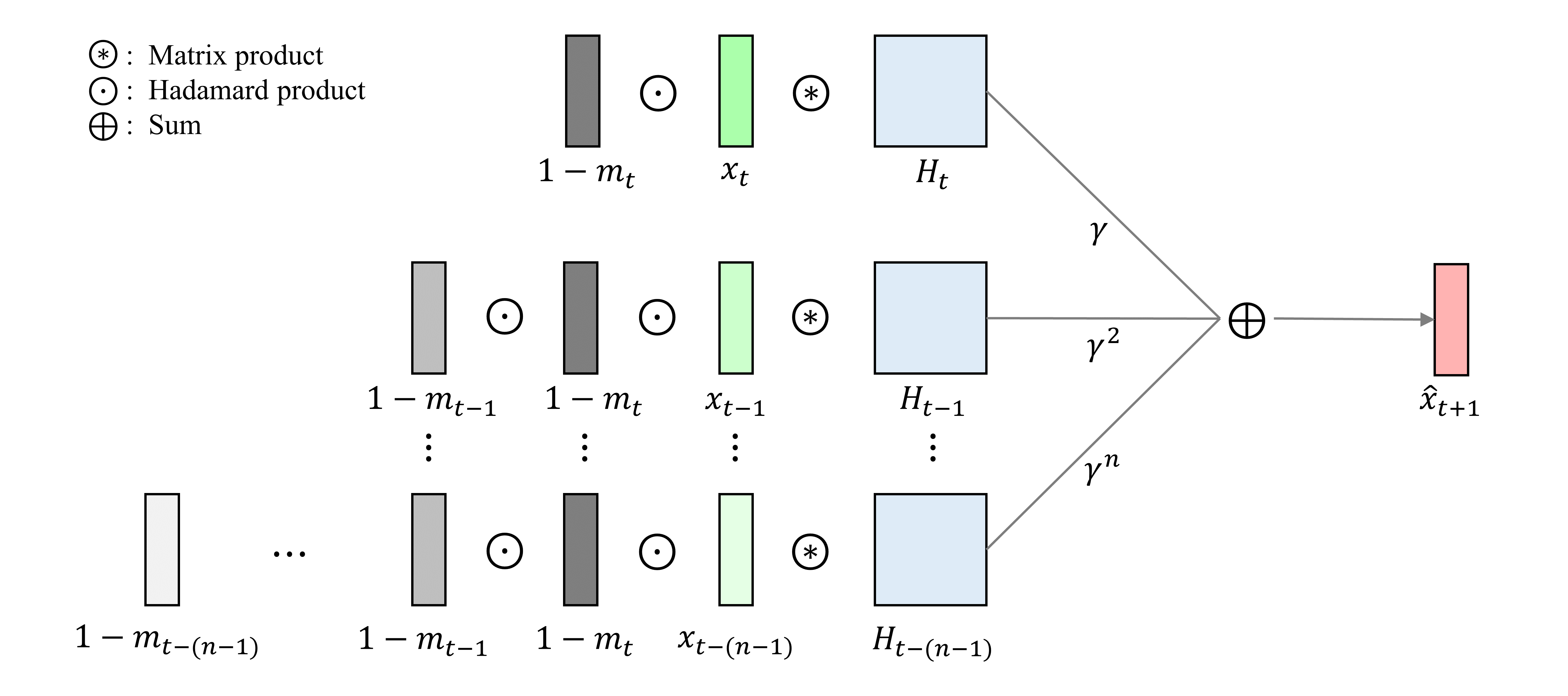
$\begin{aligned} \tilde{x}_ {t+1} &= \gamma H_t x_t \\ &+ \gamma^2 H_t H_{t-1} (x_{t-1} \odot (1-m_t)) \\ &+ \gamma^3 H_t H_{t-1} H_{t-2} (x_{t-2}\odot (1-m_ {t-1}) \odot (1-m_t)) + \cdots \\ &+ \gamma^{n} H_t \cdots H_{t-(n-1)} (x_{t-(n-1)} \odot (1-m_{t-(n-2)}) \odot \cdots \odot (1-m_t)) \\ &+ \gamma^{n} H_t \cdots H_{t-(n-1)} (\tilde{x}_ {t-(n-1)} \odot (1-m_{t-(n-1)}) \odot \cdots \odot (1-m_t)) \end{aligned}$

The $n$ steps of historical steps of states can be written in a summation form as

$\begin{aligned} \tilde{x}_ {t+1} &= \sum_{i=0}^{n-1} \gamma^{i+1} (\prod_{j=0}^{i} H_{t-j}) (x_{t-i} \odot \bigodot_{j=0}^{i-1} (1-m_{t-j})) \\ &+ \gamma^{n} H_t \cdots H_{t-(n-1)} (\tilde{x}_ {t-(n-1)} \odot (1-m_{t-(n-1)}) \odot \cdots \odot (1-m_t)) \end{aligned}$

where $\sum$ , $\prod$ , and $\bigodot$ are the summation, matrix product, and Hadamard product operators, respectively. For simplicity, we denote the term with the $\tilde{x}_{t-n-1}$ as $\mathcal{O}(\tilde{x}_{t-n-1})$ , and the GMP of the complected states can be represented by

$\tilde{x}_{t+1} = \sum_{i=0}^{n-1} \gamma^{i+1} (\prod_{j=0}^{i} H_{t-j}) (x_{t-i} \odot \bigodot_{j=0}^{i-1} (1-m_{t-j})) + \mathcal{O}(\tilde{x}_ {t-(n-1)})$

When $n$ is large enough, we consider $\mathcal{O}(\tilde{x}_ {t-(n-1)})$ is a negligibly term.

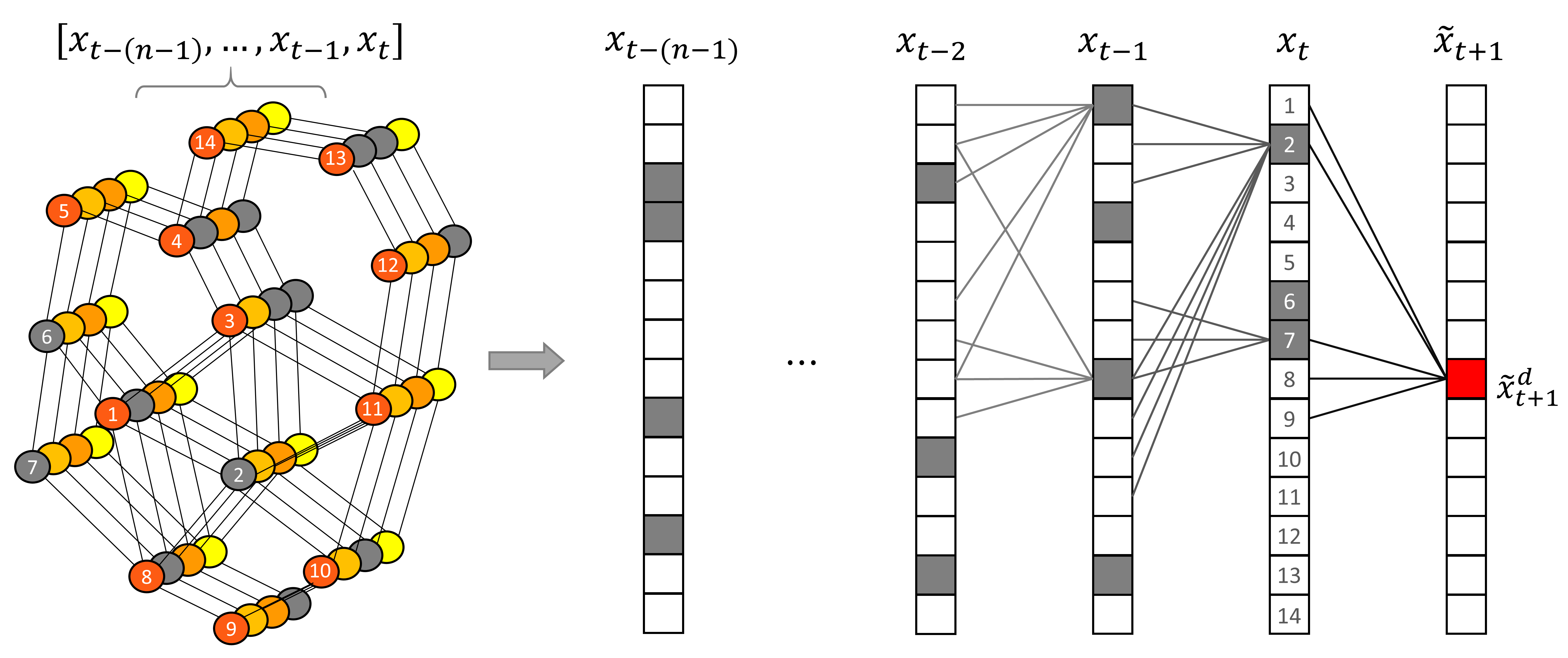
The graph Markov process can be demonstrated by the following figure. The gray-colored nodes in the left sub-figure demonstrate the nodes with missing values. Vectors on the right side represent the traffic states. The traffic states at time $t$ are numbered to match the graph and the vector. The future state (in red color) can be inferred from their neighbors in the previous steps.

GMP

The graph Markov network (GMN) is designed based on the graph Markov process, which contains $n$ transition weight matrices. The product of the these matrices $(\prod_{j=0}^{i} H_{t-j}) = (\prod_{j=0}^{i} \mathbf{A}^j \odot P_{t-j})$ measures the contribution of $x_{t-i}$ for generating the $\tilde{x}_ t$ . To reduce matrix product operations and at the same time keep the learning capability in the GMP, $(\prod_ {j=0}^{i} \mathbf{A}^j \odot P_{t-j})$ is simplified into $(\mathbf{A}^{i+1} \odot W_{i+1})$ , where $W_{i+1} \in \mathbb{R}^{S \times S}$ is a weight matrix. In this way, $(\mathbf{A}^{i+1} \odot W_{i+1})$ can directly measure the contribution of $x_{t-i}$ for generating the $\tilde{x}_ t$ and skip the intermediate state transition processes. Further, the GMP still has $n$ weight matrices ( $\{\mathbf{A}^1 \odot W_1, ..., \mathbf{A}^n \odot W_n\}$ ), and thus, the learning capability in terms of the size of parameters does not change. The benefits of the simplification is that the GMP can reduce $\frac{n(n-1)}{2}$ times of multiplication between two $S\times S$ matrices in total. The $\mathcal{O}(\tilde{x}_ {t-(n-1)})$ is considered small enough and omitted for simplicity.

Based on the GMP and the aforementioned simplification, the Graph Markov Network for traffic forecasting with missing values can be defined as

$\hat{x}_{t+1} = \sum_{i=0}^{n-1} \gamma^{i+1} (\mathbf{A}^{i+1} \odot W_{i+1}) (x_{t-i} \odot \bigodot_{j=0}^{i-1} (1-m_{t-j}))$

where $\hat{x}_ {t+1}$ is the predicted traffic state for the future time step $t+1$ and $\{W_1,...,W_n\}$ are the model’s weight matrices that can be learned and updated during the training process.

Structure of the graph Markov network is shown below. Here, $H_{t-j} = \mathbf{A}^j\odot W_j$ .

GMN

Code

The code for implementing the GMN is published in this GitHub Repo.

Reference

For more details of the model and experimental results, please refer to

[1] Zhiyong Cui, et al. Graph markov network for traffic forecasting with missing data. Transportation Research Part C: Emerging Technologies, 2020. [arXiv]